Sunday, 9 October 2022

ASCE 7-10 Wind Load Calculation Example


ASCE 7-10 Wind Load Calculation Example

A fully worked example of ASCE 7-10 wind load calculations

SkyCiv released a free wind load calculator that has several code references including the ASCE 7-10 wind load procedure. In this section, we are going to demonstrate how to calculate the wind loads, by using an S3D warehouse model below:

ASCE 7-10 Wind load calculation

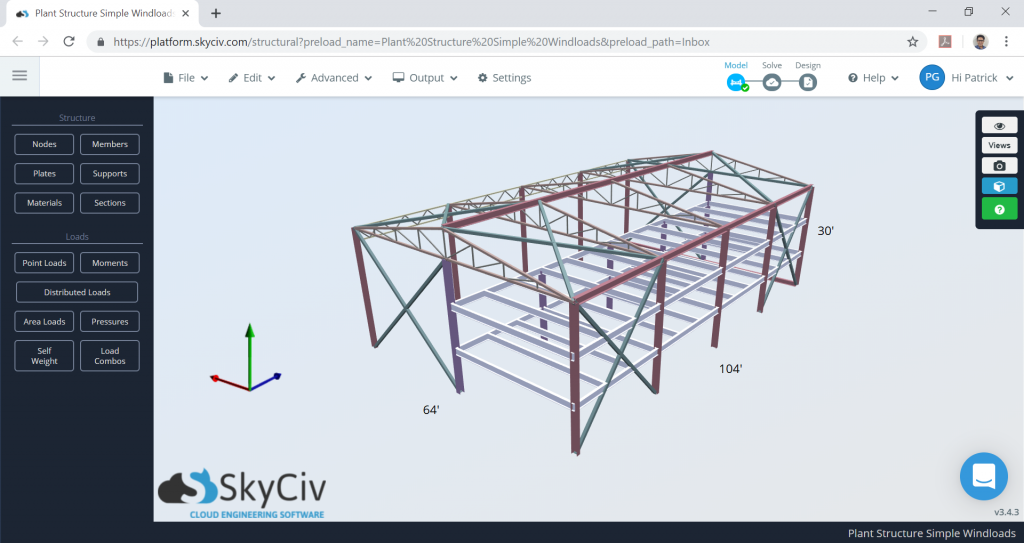
Figure 1. Warehouse model in SkyCiv S3D as an example.

ASCE 7-10 Wind load calculation

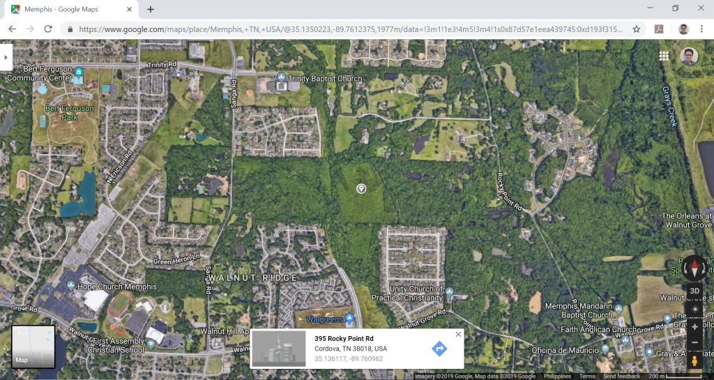
Figure 2. Site location (from Google Maps).

Table 1. Building data needed for our wind calculation.

LocationCordova, Memphis, Tennessee
OccupancyMiscellaneous – Plant Structure
TerrainFlat farmland
Dimensions64 ft × 104 ft in plan
Eave height of 30 ft
Apex height at elev. 36 ft
Roof slope 3:16 (10.62°)
With opening
CladdingPurlins spaced at 2ft
Wall studs spaced at 2ft


In our ASCE 7-10 wind load example, design wind pressures for a large, three-story plant structure will be determined. Fig. 1 shows the dimensions and framing of the building. The building data are shown in Table 1.

Although there are a number of software that have wind load calculation already integrated into their design and analysis, only a few provide a detailed computation of this specific type of load. Users would need to conduct manual calculations of this procedure in order to verify if the results are the same as those obtained from the software.

The formula in determining the design wind pressure are:

For enclosed and partially enclosed buildings:

p=qGCpqi(GCpi)     (1)

For open buildings: 

p=qGfCpq(GCpi)     (2)

Where:

G = gust effect factor
Cp = external pressure coefficient
(GCpi)= internal pressure coefficient
q = velocity pressure, in psf, given by the formula:

q=0.00256KzKztKdV2     (3)

q = qh for leeward walls, side walls, and roofs,evaluated at roof mean height, h
q = qz for windward walls, evaluated at height, z
qi = qh for negative internal pressure, (GCpi) evaluation and qz for positive internal pressure evaluation (+GCpi) of partially enclosed buildings but can be taken as qh for conservative value.
Kz = velocity pressure coefficient
Kzt= topographic factor
Kd= wind directionality factor
V = basic wind speed in mph

We will dive deep into the details of each parameter below. Moreover, we will be using the Directional Procedure (Chapter 30 of ASCE 7-10) in solving the design wind pressures.

Risk Category

The first thing to do in determining the design wind pressures is to classify the risk category of the structure which is based on the use or occupancy of the structure. For this example, since this is a plant structure, the structure is classified as Risk Category IV. See Table 1.5-1 of ASCE 7-10 for more information about risk categories classification.

Basic Wind Speed, V

The ASCE 7-10 provides a wind map where the corresponding basic wind speed of a location can be obtained from Figures 26.5-1A to 1C. The Occupancy Category is defined and classified in the International Building Code.

When viewing the wind maps, take the highest category number of the defined Risk or Occupancy category. In most cases, including this example, they are the same. From Figure 26.5-1B, Cordova, Memphis, Tennessee is somehow near where the red dot on Figure 3 below, and from there, the basic wind speed, V, is 120 mph. Take note that for other locations, you would need to interpolate the basic wind speed value between wind contours.

ASCE 7-10 Wind load calculation

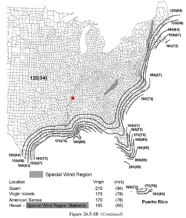
Figure 3. Basic wind speed map from ASCE 7-10.

SkyCiv now automates the wind speed calculations with a few parameters. Try our SkyCiv Free Wind Tool

Exposure Category

See Section 26.7 of ASCE 7-10 details the procedure in determining the exposure category.

Depending on the wind direction selected, the exposure of the structure shall be determined from the upwind 45° sector. The exposure to be adopted should be the one that will yield the highest wind load from the said direction.

The description of each exposure classification is detailed in Section 26.7.2 and 26.7.3 of ASCE 7-10. To better illustrate each case, examples of each category are shown in the table below.

Table 2. Examples of areas classified according to exposure category (Chapter C26 of ASCE 7-10).

EXPOSUREEXAMPLE
Exposure B
  • Suburban residential area with mostly single-family dwellings – Low-rise structures, less than 30 ft high, in the center of the photograph have sites designated as exposure b with surface roughness Category B terrain around the site for a distance greater than 1500 ft in any wind direction.
  • An urban area with numerous closely spaced obstructions having the size of single-family dwellings or larger – For all structures shown, terrain representative of surface roughness category b extends more than twenty times the height of the structure or 2600 ft, whichever is greater, in the upwind direction. Structures in the foreground are located in exposure B – Structures in the center top of the photograph adjacent to the clearing to the left, which is greater than approximately 656 ft in length, are located in exposure c when the wind comes from the left over the clearing.
Exposure C
  • Flat open grassland with scattered obstructions having heights generally less than 30 ft.
  • Open terrain with scattered obstructions having heights generally less than 30 ft for most wind directions, all 1-story structures with a mean roof height less than 30 ft in the photograph are less than 1500 ft or ten times the height of the structure, whichever is greater, from an open field that prevents the use of exposure B.
Exposure D
  • A building at the shoreline (excluding shorelines in hurricane-prone regions) with wind flowing over open water for a distance of at least 1 mile. Shorelines in exposure D include inland waterways, the great lakes, and coastal areas of California, Oregon, Washington, and Alaska.


For our example, since the location of the structure is in farmland in Cordova, Memphis, Tennessee, without any buildings taller than 30 ft, therefore the area is classified as 
Exposure C. A helpful tool in determining the exposure category is to view your potential site through a satellite image (Google Maps for example).

Wind Directionality Factor, Kd

The wind directionality factors, Kd, for our structure are both equal to 0.85 since the building is the main wind force resisting system and also has components and cladding attached to the structure. This is shown in Table 26.6-1 of ASCE 7-10 as shown below in Figure 4.

ASCE 7-10 Wind load calculation

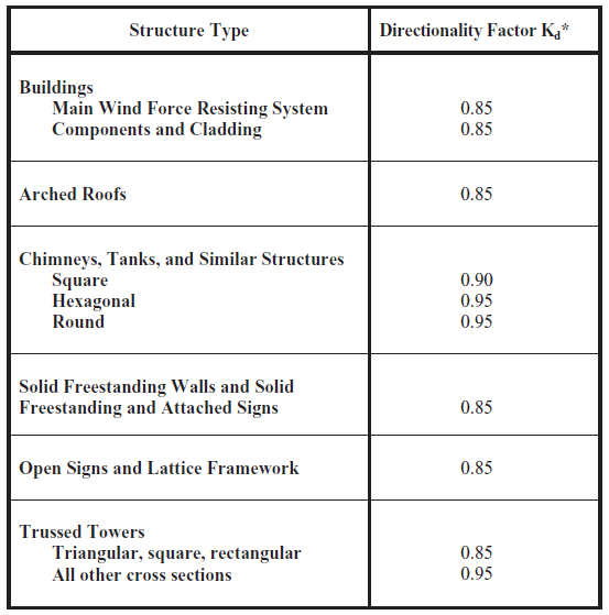
Figure 4. Wind directionality factor based on structure type (Table 26.6-1 of ASCE 7-10).

Topographic Factor, Kzt

Since the location of the structure is in flat farmland, we can assume that the topographic factor, Kzt, is 1.0. Otherwise, the factor can be solved using Figure 26.8-1 of ASCE 7-10. To determine if further calculations of the topographic factor are required, see Section 26.8.1, if your site does not meet all of the conditions listed, then the topographic factor can be taken as 1.0.

ASCE 7-10 Wind load calculation

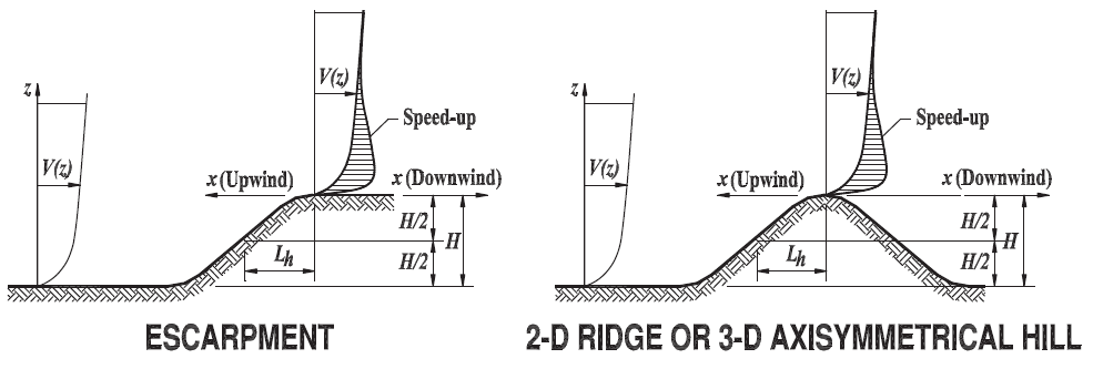
Figure 5. Parameters needed in calculation topographic factor, Kzt (Table 26.8-1 of ASCE 7-10).

Note: Topography factors can automatically be calculated using SkyCiv Wind Design Software

Velocity Pressure Coefficient, Kz

The velocity pressure coefficient, Kz, can be calculated using Table 27.3-1 of ASCE 7-10. This parameter depends on the height above ground level of the point where the wind pressure is considered, and the exposure category. Moreover, the values shown in the table is based on the following formula:

For 15ft < z < zg: Kz=2.01(z/zg)2/α     (4)
For z < 15ft: Kz=2.01(15/zg)2/α     (5)

Where:

Table 3. Values of and zg from table 26.9-1 of ASCE 7-10.

Exposureαzg(ft)
B71200
C9.5900
D11.5700


Usually, velocity pressure coefficients at the mean roof height, Kh
, and at each floor level, Kzi, are the values we would need in order to solve for the design wind pressures. For this example, since the wind pressure on the windward side is parabolic in nature, we can simplify this load by assuming that uniform pressure is applied on walls between floor levels.

The plant structure has three (3) floors, so we will divide the windward pressure into these levels. Moreover, since the roof is a gable-style roof, the roof mean height can be taken as the average of roof eaves and apex elevation, which is 33 ft.

Table 4. Calculated values of velocity pressure coefficient for each elevation height.

Elevation (ft)Kz
100.85
200.90
300.98
331.00 Kzh

Velocity Pressure

From Equation (3), we can solve for the velocity pressure, q in PSF, at each elevation being considered.

Table 5. Calculated values of velocity pressure at each elevation height.

Elevation (ft)Kzq(psf)Remarks
100.8526.631st floor
200.9028.202nd floor
300.9830.71Roof eave
331.0031.33Roof mean height, qh

Gust Effect Factor, G

The gust effect factor, G, is set to 0.85 as the structure is assumed rigid (Section 26.9.1 of ASCE 7-10).

Enclosure Classification and Internal Pressure Coefficient

The plant structure is assumed to have openings that satisfy the definition of a partially enclosed building in Section 26.2 of ASCE 7-10. Thus, the internal pressure coefficient, (GCpi), shall be +0.55 and -0.55 based on Table 26.11-1 of ASCE 7-10.

ASCE 7-10 Wind load calculation

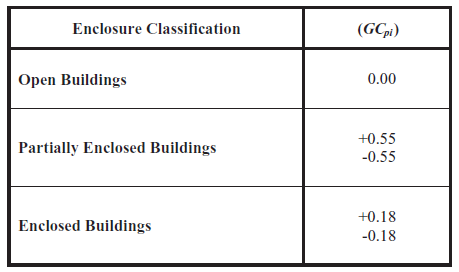
Figure 6. Internal Pressure Coefficient, (GCpi), from Table 26.11-1of ASCE 7-10.

External Pressure Coefficient, Cp

For enclosed and partially enclosed buildings, the External Pressure Coefficient, Cpis calculated using the information provided in Figure 27.4-1 through Figure 27.4-3. For a partially enclosed building with a gable roof, use Figure 27.4-1.

External Pressure Coefficients for the walls and roof are calculated separately using the building parameters L, B, and h, which are defined in Note 7 of Figure 27.4-1.

Thus, we need to calculate the L/B and h/L:

Roof mean height, h = 33′
Building length, L = 64′
Building width, B = 104′
L/B = 0.615
h/L = 0.516
h/B = 0.317

From these values, we can obtain the external pressure coefficients, Cp, for each surface using table 27.4-1 of ASCE 7-10. Take note that we can use linear interpolation when roof angle, θ, L/B, and h/L values are in between those that are in the table. For our example, the external pressure coefficients of each surface are shown in Tables 6 to 8.

Table 6. Calculated external pressure coefficients for wall surfaces.

SurfaceCp
Windward wall0.8
Leeward wall-0.5
Side wall-0.7


Table 7. Calculated external pressure coefficients for roof surfaces (wind load along L).

External pressure coefficients for roof Cp (along L)
h/LWindwardLeeward
10°10.62°15°10°10.62°15°
0.5-0.9
-0.18
-0.88
-0.18
-0.7
-0.18
-0.50-0.50-0.50
0.516-0.91
-0.18
-0.89
-0.18
-0.71
-0.18
-0.51-0.51-0.50
1.0-1.3
-0.18
-1.26
-0.18
-1.0
-0.18
-0.70-0.69-0.60


Table 8. Calculated external pressure coefficients for roof surfaces (wind load along B).

External pressure coefficients for roof Cp (along B)
h/BLocationCp
0.3170 to h-0.9
-0.18
h/2 to h-0.9
-0.18
h to 2h-0.5
-0.18
>2h-0.3
-0.18


External pressure coefficient with two values as shown in Tables 7 and 8 shall be checked for both cases.

Design Wind Pressures for Main Wind Frame Resisting System

Using Equation (1), the design wind pressures can be calculated. Results of our calculations are shown on Tables 8 and 9 below. Take note that there will be four cases acting on the structure as we will consider pressures solved using (+GCpi) and (GCpi) , and the +Cp  and Cp  for roof.

Table 9. Design wind pressure for wall surfaces.

Design Pressure, p, for Walls
Floor elevationqz, psfWindwardLeewardSide wall
(+GCpi)(GCpi)(+GCpi)(GCpi)(+GCpi)(GCpi)
1026.630.88 (0.88)35.35 (35.35)-30.55
(-30.55)
3.92
(3.92)
-35.88
(-35.88)
-1.41
(-1.41)
2028.201.94 (1.94)36.41 (36.41)
3030.713.65 (3.65)38.12 (38.12)
3331.334.07 (4.07)38.54 (38.54)

(SkyCiv Wind Load results)

Table 10. Design wind pressure for roof surfaces.

Design Roof Pressure, psf (along L)Design Roof Pressure, psf (along B)
Surface(+GCpi)(GCpi)Location
(from windward edge)
(+GCpi)(GCpi)
Windward-40.87 (-40.87)-6.41 (-6.40)0 to h/2-41.20(-41.20)12.44(12.44)
-22.03 (-22.03)12.44 (12.44)h/2 to h-41.20(-41.20)
Leeward-30.71 (-30.71)3.76 (3.83)h to 2h-30.55(-30.55)
>2h-25.22(-25.22)

(SkyCiv Wind Load results)

To apply these pressures to the structure, we will consider a single frame on the structure. Sample of applying case 1 and 2 (for both (GCpi)) are shown in  Figures 7 and 8. The wind direction shown in the aforementioned figures is along the length, L, of the building.

Take note that a positive sign means that the pressure is acting towards the surface while a negative sign is away from the surface. Bay length is 26 feet.

ASCE 7-10 Wind load calculation

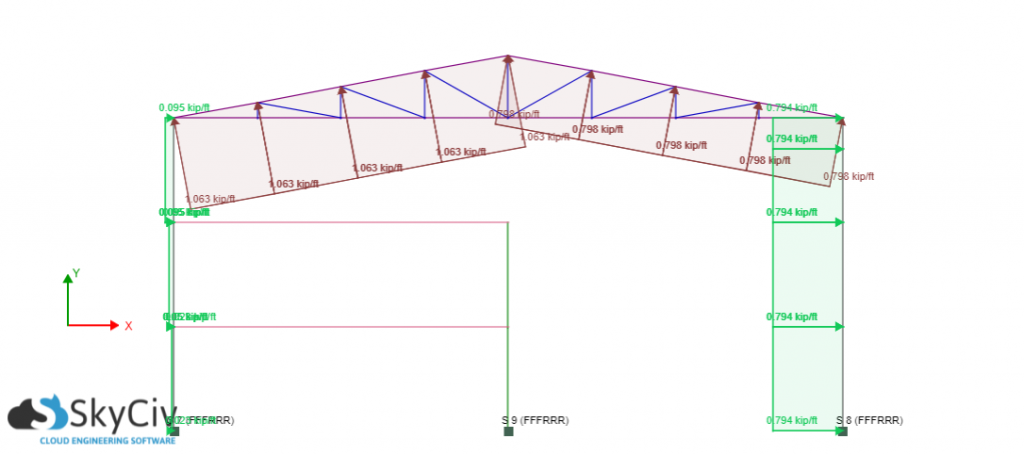
Figure 7. Design wind pressure applied on one frame – (+GCpi) and absolute max roof pressure case.

ASCE 7-10 Wind load calculation

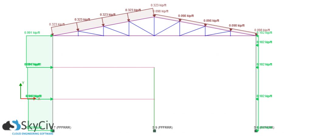
Figure 8. Design wind pressure applied on one frame – (GCpi) and absolute max roof pressure case.

SkyCiv simplifies this procedure by just defining parameters. Try our SkyCiv Free Wind Tool

Design Wind Pressures for Components and Cladding (C&C)

Components and claddings are defined in Chapter C26 of ASCE 7-10 as: “Components receive wind loads directly or from cladding and transfer the load to the MWFRS” while “cladding receives wind loads directly.” Examples of components include “fasteners, purlins, studs, roof decking, and roof trusses” and for cladding are “wall coverings, curtain walls, roof coverings, exterior windows, etc.”

From Chapter 30 of ASCE 7-10, design pressure for components and cladding shall be computed using the equation (30.4-1), shown below:

p=qh[(GCp)(GCpi)]     (6)

Where:

qh: velocity pressure evaluated at mean roof height, h (31.33 psf)
(GCpi): internal pressure coefficient
(GCp): external pressure coefficient

For this example, (GCp) will be found using Figure 30.4-1 for Zone 4 and 5 (the walls), and Figure 30.4-2B for Zone 1-3 (the roof). In our case, the correct figure used depends on the roof slope, θ, which is 7°< θ ≤ 27°. (GCp) can be determined for a multitude of roof types depicted in Figure 30.4-1 through Figure 30.4-7 and Figure 27.4-3 in Chapter 30 and Chapter 27 of ASCE 7-10, respectively.

We shall only calculate the design wind pressures for purlins and wall studs. Zones for components and cladding pressures are shown in Figure 9.

ASCE 7-10 Wind load calculation

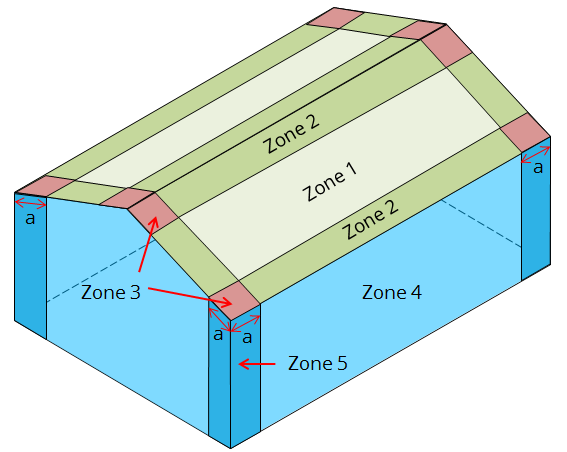
Figure 9. Location of calculated C&C pressures.

The distance a from the edges can be calculated as the minimum of 10% of least horizontal dimension or 0.4h but not less than either 4% of least horizontal dimension or 3 ft.

a : 10% of 64ft = 6.4 ft > 3ft
0.4(33ft) = 13.2 ft 4% of 64ft = 2.56 ft
a = 6.4 ft

Wall Studs (C&C Wall Pressure)

Based on Figure 30.4-1, the (GCpcan be calculated for zones 4 and 5 based on the effective wind area. Take note that the definition of effective wind area in Chapter C26 of ASCE 7-10 states that: “To better approximate the actual load distribution in such cases, the width of the effective wind area used to evaluate (GCp) need not be taken as less than one-third the length of the area.” Hence, the effective wind area should be the maximum of:

Effective wind area = 10ft*(2ft) or 10ft*(10/3 ft) = 20 sq.ft. or  33.3 sq ft.
Effective wind area = 33.3 sq ft.

The positive and negative (GCp) for walls can be approximated using the graph shown below, as part of Figure 30.4-1:
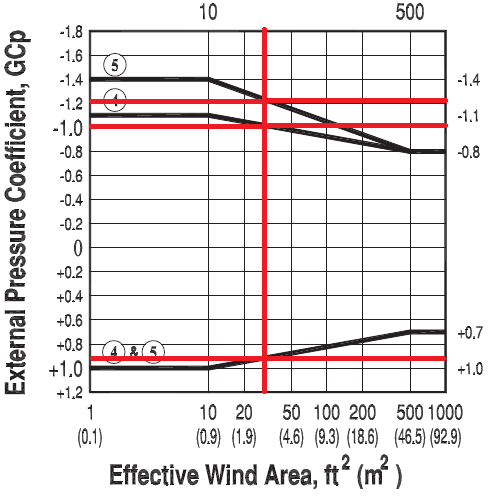
ASCE 7-10 Wind load calculation

Figure 10. Approximated (GCp) values from Figure 30.4-1 of ASCE 7-10.

Table 11. Calculated C&C pressures for wall stud.

Zone+(GCp)(GCp)C&C Pressures, psf
+(GCp)(GCp)
40.90-1.010.97
45.43
-48.56
-14.10
50.90-1.210.97
45.43
-54.83
-20.36

Purlins (C&C Roof Pressure)

From 30.4-2B, the effective wind pressures for Zones 1, 2, and 3 can be determined. Since trusses are spaced at 26ft, hence, this will be the length of purlins. The effective wind area should be the maximum of:

Effective wind area = 26ft*(2ft) or 26ft*(26/3 ft) = 52 ft2 or  225.33 sq.ft.
Effective wind area = 225.33 sq.ft.

The positive and negative (GCp) for the roof can be approximated using the graph shown below, as part of Figure 30.4-2B:
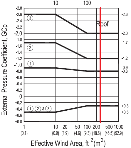
ASCE 7-10 Wind load calculation

Figure 11. (GCp) values from Figure 30.4-2B of ASCE 7-10.

Table 12. Calculated C&C pressures for purlins.

Zone+(GCp)-(GCp)C&C Pressures, psf
+(GCpi)-(GCpi)
10.30-0.80-7.83
26.63
-42.30
-7.83
20.30-1.2-7.83
26.63
-54.83
-20.36
30.30-2.0-7.83
26.63
-79.89
-45.43

These calculations can be all be performed using SkyCiv’s Wind Load Software for ASCE 7-10, 7-16, EN 1991, NBBC 2015, and AS 1170. Users can enter in a site location to get wind speeds and topography factors, enter in building parameters and generate the wind pressures. With a Professional Account, users can auto-apply this to a structural model and run structural analysis all in one software.

Otherwise, try our SkyCiv Free Wind Tool for wind speed and wind pressure calculations on simple structures.


References:

  • Mehta, K. C., & Coulbourne, W. L. (2013, June). Wind Loads: Guide to the Wind Load Provisions of ASCE 7-10. American Society of Civil Engineers.
  • Minimum Design Loads for Buildings and Other Structures. (2013). ASCE/SEI 7-10. American Society of Civil Engineers.
Thanks to 
Patrick Aylsworth Garcia Structural Engineer, Product Development
Patrick Aylsworth Garcia
Structural Engineer, Product Development
MS Civil Engineering


                 Er. SP.ASWINPALANIAPPAN., M.E.,(Strut/.,)
Structural Engineer

Thursday, 6 October 2022

A Computational study on buckling behavior of cold-formed steel built-up columns using compound spline finite strip method

 A Computational study on buckling behavior of cold-formed steel built-up columns using compound spline finite strip method


This paper presents a computational methodology to compute the critical buckling stress of built-up cold-formed steel columns joined with discrete fasteners. The fasteners are modeled as three-dimensional beam elements, and their effect is integrated into the spline finite strip framework, evolving the compound strip methodology. Although this technique has been presented in the literature, this paper presents yet another robust framework for the buckling load evaluation of compound cold-formed steel columns with arbitrarily located fasteners. The proposed framework is applied to study the effect of fasteners on the formation of local, distortional, and global buckling modes of built-up section and a comparison is drawn with the buckling behavior of a single section. In this study, the proposed formulations are also used to get insights into the stability behavior of single-span and multi-span compound cold-formed steel columns in the presence of (i) fasteners with varied spacing's with respect to span and (ii) the presence of the additional restraining system such as wall panels. For different buckling modes, a significant increment in buckling stress for a built-up section from a single section is observed when the fastener spacing is kept less than the critical buckling half-wavelength of the respective buckling modes. The study on the effect of wall panels shows that in comparison to unsheathed wall studs, the sheathed wall studs that produce additional constraints lead to the elimination of the global buckling deformations. The proposed formulations are simple, yet rigorous and have been validated using finite element-based numerical results.

Keywords: spline finite strip method; cold-formed steel; built-up section; buckling analysis 

Thanks to 

Akshay Mangal Mahar, S Arul Jayachandran

Journal International Journal of Structural Stability and Dynamics 

Er. SP.ASWINPALANIAPPAN., M.E.,(Strut/.,)
Structural Engineer

JOINT DETAILING OF STEEL CONCAVE SECTIONS ( Steel Design)

 JOINT DETAILING OF STEEL CONCAVE SECTIONS  ( Steel Design)


* JOINT DETAILING OF STEEL Concave SECTIONS *

Detailing of joints in sword structure is as important important as detailing of main structural members. Eventually loads from structures are transferred to different structural members through joints. So, a good detailing of joints in sword structure is needed to make the structure safe for the given loads.


Then we will bandy about the types of joints generally used for structural sword concave sections. Concave sections are of three types, Blockish Concave Sections( RHS) and Square Hollow Sections( SHS) and indirect Concave Sections( CHS).

Following are the common details for structural sword concave sections( RHS and SHS) generally used

1. K – Type Joints

K – Type joints in sword structures are formed when the centroidal axis of vertical member and two side bracing s meet with the central axis of top passion. Following figure shows K- Type joint

It should be assured that the ends of concave sections are always closed.However, also a plate is welded on that end so that the ends gets unrestricted and also the connection with other members are made good by effective sealing of the members, If any ends of a concave section doesn't get closed due to further range. This also prevents internal erosion of the concave sections.

K- type of joints in structural sword members is simplest and most provident.

2. Knee – Type Joint

To increase the stability of connection between perpendicular and vertical members of structure, knee- type joint is used.

In welded knee- joint, the top passion is directly welded to the main column and also a suitably cut haunch is welded to the perpendicular and as well as to the passion member for better stiffening. The knee- type joint is shown below

3. N – Type Joint

N- type joint is formed as per the espoused configuration, for connecting web members to top and nethermost passions. Typical details of one of the joints are given below

i) In this joint, first the perpendicular member is put in place and directly welded to top and nethermost passions.

ii) latterly, the other inclined slant member, with suitable double cuts at the ends, is directly welded to top and nethermost passions and also to the perpendicular.

iii) These connections, of perpendicular and slant members to eclipse and nethermost passions directly, help in barring the gusset plates therefore performing in automatic sealing of member ends. Direct jointing, of perpendicular and slant members to eclipse and nethermost passions, eliminates gusset plates.


Er. SP.ASWINPALANIAPPAN., M.E.,(Strut/.,)
Structural Engineer

WHY BIM IS AN ESSENTIAL PART FOR GREEN BUILDING REVOLUTION?

 WHY BIM IS AN ESSENTIAL PART FOR GREEN BUILDING REVOLUTION?


The world is just not sustainable at the current rate. And that's why every sector is laboriously sharing in this green revolution. And speaking of involvement, the construction sector is responsible for 37 of carbon emigrations( finds UN report – wisdomNews.20- Oct- 2021). This number is scary enough for the AEC assiduity to significantly contribute to global sustainability through aware designs.

And to reduce the implicit detriment from the conduct of the AEC assiduity, they introduced “ Green structure. “ This frame is an essential guideline in sustainability because it takes a comprehensive look at the implicit consequences of reckless construction.

Green structure is an energy-effective construction strategy that results in healthier structures that have a lower environmental effect and bring lower to maintain. This environmentally friendly construction system considers the entire life cycle of a structure, including sitting, design, construction, operation, conservation, restoration, and destruction. Sustainable design includes green armature, but it also addresses challenges ranging from the micro( sustainable cabinetwork design) to the macro( sustainable civic planning).

WHY IS THE APPROACH OF GREEN BUILDING A MUST FOR THE AEC Assiduity?

The Green Building, in design, construction or operation, reduces or eliminates negative impacts and can produce positive results. This requires close cooperation of the contractor, engineers, masterminds, and the customer at all design stages. And BIM comes into play.

BIM as a technology( Building Information Modelling) contributes significantly to the Architectural Engineering and Construction( AEC) business. BIM promotes the design, construction, and operating processes by using participated digital representations of erecting means as a secure foundation for decision- timber. It can model the design in three confines( 3D), manage the design timeline, and allow construction workers to check and check structures throughout their lifetime.

And BIM, as an essential tool in green structure, is game- changing. It enables new situations of design perfection, serving both the terrain and the construction sector. Through sustainable, green structure design ways and workflows, a green structure developed with BIM services gives a better terrain for analysis and decision- timber.

GREEN BUILDING VIA BIM

BIM software like Revit, AutoCAD Architecture and MEP, and Navisworks may give a whole- structure analysis, letting contrivers understand energy costs for fiscal and design opinions. Contrivers and contractors can use BIM software to pretend energy law compliance. Whole- structure assessments incorporate meteorological data, allowing contrivers to use literal climatic information when developing a calibrated energy model.

We indeed support the frame of Green design in the construction assiduity. The discussion between the American Institute of Engineers Committee on the terrain( AIA/ Pen) and the United States Green Building Council( USGBC) indicates the increased emphasis on green or sustainable design.

We hope we've clear the conception of Green Building and green design through BIM. Now let’s briefly understand the donation of BIM to sustainable construction.

1. RESPONSIVENESS DURING THE DESIGN PHASE

The participated model function in BIM software allows everyone involved in the design to pierce the model fluently.

It promotes translucency in the process. It allows them to get real- time data on recommended particulars and accouterments .

The translucency handed then allows contractors, masterminds, suppliers, and others to advise on the entire design and operation of the structure beforehand on, giving bettered sustainability before any plutocrat is spent. Only ecologically friendly products and processes are used, and time and plutocrat are saved on revamping and cataloging . Further, The entire platoon may contribute their experience and moxie to find a long- term BIM result.

2. Advanced effectiveness IN THE CONSTRUCTION PHASE

Before the invention of BIM, it was challenging to maintain the data about any architectural revision intermittently throughout the construction phase.

But now, it’s not the case presently, as the 3D models handed by BIM have streamlined real- time data participating at every process step. It also allows the platoon to review the workflow and ameliorate if demanded.

This improves effectiveness by saving time through clash discovery and thereby lowering the total threat of mortal crimes or the demand for rework. This saves coffers, reduces waste, and pets up work, contributing to a lower environmental imprint.

And formerly the structure is functional, the structure proprietor or director can carry out conservation work more efficiently. This optimises the structure’s continuing resource use and, as a result, its environmental impact.

The global movement to be more environmentally responsible is catching the construction assiduity, and BIM armature is the way forward.

3. STRONGER COMMAND DURING THE product PHASE

Another substantial benefit of using BIM in green structures is that with 3D models, a installation’s continuing operations can be significantly optimised.

All stakeholders may help the unanticipated event with readily available data on upgrades, refurbishments, and renewals.

farther, more construction experts, masterminds & engineers are using this factor by incorporating long- term, environmentally responsible functional advice and conservation plans into their final design parameters. This adds value to structure possessors and enhances overall sustainability.

4. GREEN BUILDING instrument

LEED Certified Sustainable Green Building Design has the implicit to come a reality in the structure assiduity thanks to BIM. LEED, which stands for Leadership in Energy and Environmental Design, is one of the world’s most generally utilised green structure standing systems.

Using BIM technology, AEC professionals bring the sustainable design of a green structure to construction. 3D Revit BIM Models give shop delineations that can be participated with the construction crew.

CONCLUSION

The engineers were backed by BIM modeling how solar ways, water systems, and the structure’s figure affect ventilation. The construction was intended to operate with the wind pattern, with ventilation and tailwind analysed and estimated using BIM.

It’s not surprising that BIM technologies like Revit, AutoCAD Architecture and MEP, and Navisworks may vastly ameliorate the simplicity of planning and enforcing sustainable practices during the structure design process.


Er. SP.ASWINPALANIAPPAN., M.E.,(Strut/.,)
Structural Engineer

SEISMIC RELIABILITY OF CHEVRON BRACED FRAMES WITH INNOVATIVE CONCEPT OF BRACING MEMBERS

 SEISMIC RELIABILITY OF CHEVRON BRACED FRAMES WITH INNOVATIVE CONCEPT OF BRACING MEMBERS 


ABSTRACT: 

    According to the most modern trend, performance-based seismic design is aimed at the evaluation of the seismic performance of structures in terms of mean annual frequency of exceeding a threshold level of damage, i.e. a limit state. A procedure for performance-based seismic assessment is herein briefly summarized and applied to concentrically “V” braced steel frames, designed according to different criteria. In particular, two design approaches are examined. The first one corresponds to the provisions suggested by Euro-code 8, while the second approach, proposed by the authors, is based on a rigorous application of the capacity design criteria aiming at the control of the failure mode. In addition in this work a new conception of bracing members is developed and applied with reference to V-braced frames designed according to the methodology proposed by the authors.  It is well known that aiming at the safeguard of brace connections, Euro-code 8 provides a limitation to the brace slenderness. The drawback of this limitation is the over-sizing of brace diagonals at the upper storeys, which prevents the development of a collapse mechanism of global type. 

    This is the starting design issue for the conception of new bracing members. In fact, by introducing in the brace members a zone characterized by a reduction of the cross sectional area (Reduced Section Solution), it is possible to calibrate the yield strength leaving substantially unchanged the slenderness, so that the limits provided for the normalized slenderness can be still satisfied without brace over-sizing.  The aim of this work is to focus on the seismic performance of V-braced frames designed according to both Euro-code provisions and the proposed methodology.

     For the structures dimensioned according to the proposed criteria, the Reduction Section Solution is also applied with the aim to safeguard the connection without increasing the structural weight. Finally, a probabilistic approach based on the combination of probabilistic seismic hazard analysis (PSHA), probabilistic seismic demand analysis (PSDA) and probabilistic seismic capacity analysis (PSCA) is applied aiming to investigate the seismic performance of the designed structures. 

    It is pointed out how the proposed design method leads to a very important improvement of the seismic performances with a negligible increase of the overall building cost. 

Keywords: Seismic reliability; concentrically braced frames; seismic hazard; probabilistic seismic demand Analysis; structural capacity 

Thanks to 

A. Longo, R. Montuori and V. Piluso* 
Department of Civil Engineering, University of Salerno via Ponte Don Melillo, Fisciano, 84084, Italy *(Corresponding author: E-mail: v.piluso@unisa.it)

Er. SP.ASWINPALANIAPPAN., M.E.,(Strut/.,)
Structural Engineer

Investigations on Efficiently Interfaced Steel Concrete Composite Deck Slabs

 Investigations on Efficiently Interfaced Steel Concrete Composite Deck Slabs


        Thestrengthofthecompositedeckslabdependsmainlyonthelongitudinalsheartransfermechanismattheinterfacebetweensteel and concrete. The bond strength developed by the cement paste is weak and causes premature failure of composite deck slab. This deficiency is effectively overcame by a shear transferring mechanism in the form of mechanical interlock through indentations, embossments, or fastening studs. Development of embossment patterns requires an advanced technology which makes the deck profile expensive. Fastening studs by welding weakens the joint strength and also escalates the cost. The present investigation is attempted to arrive at a better, simple interface mechanism. Three types of mechanical connector schemes are identified and investigated experimentally. All of the three shear connector schemes exhibited full shear interaction with negligible slip. The strength and stiffness of the composite slabs with shear connectors are superior about one and half time compared to these of the conventional reinforced concrete slabs and about twice compared to these of composite slabs without mechanical shear connectors. The scheme2 and scheme3 shear connector mechanisms integrate deck webs and improve strength and stiffness of the deck, which can effectively reduce the cost of form-works and supports efficiently.

Thanks to 

K. N.Lakshmikandhan, P.Sivakumar, R. Ravichandran, and S. Arul Jayachandran 
Structural Engineering Research Centre, Council for Scientific and Industrial Research, Taramani, Chennai 600113, India 


Er. SP.ASWINPALANIAPPAN., M.E.,(Strut/.,)
Structural Engineer

Evaluation of connection flexibility in cold formed steel racks


Evaluation of connection flexibility in cold formed steel racks


Abstract

        Steel storage racks are three-dimensional framed structures fabricated from cold formed steel sections, wherein hook-in end connectors are used to make beam–column connections which are basically bolt less and semi-rigid in nature. Different types of beam end connectors with different geometry of the connected members are available, making it impossible to develop a generalized analytical model. Only very few theoretical models are available to evaluate the performance of the joints for some typical connectors. More often experimental evaluation and numerical studies are needed to predict the behavior of every different type of connectors. In the present study eighteen experiments were conducted on a commercially available pallet rack connection by varying the most influencing parameters such as thickness of the column, depth of the connector and the depth of the beam. The main objective of this work is to quantify the beam to column joint, flexibility of commonly used pallet rack frame and to develop a general Frye–Morris type/three parameter power model type moment versus relative rotation relationship. A companion finite element shell model that simulates the experimental behavior closely is developed using ABAQUS finite element software, which is also used for further parametric studies. Using the three major variables as size parameters, a Frye–Morris type of equation has been proposed. Some calibration studies have also been carried out. Using the ultimate moment capacity, initial connection stiffness and the shape parameter obtained, a three parameter power model has also been proposed to represent the moment–rotation behavior of the bolt less connections.


Thanks to 

P.Prabha

V. Marimuthu

M.Saravanan

S.Arul Jayachandran  


Er. SP.ASWINPALANIAPPAN., M.E.,(Strut/.,)
Structural Engineer